Prospects of deep learning for medical imaging
Article information
Abstract
Machine learning techniques are essential components of medical imaging research. Recently, a highly flexible machine learning approach known as deep learning has emerged as a disruptive technology to enhance the performance of existing machine learning techniques and to solve previously intractable problems. Medical imaging has been identified as one of the key research fields where deep learning can contribute significantly. This review article aims to survey deep learning literature in medical imaging and describe its potential for future medical imaging research. First, an overview of how traditional machine learning evolved to deep learning is provided. Second, a survey of the application of deep learning in medical imaging research is given. Third, wellknown software tools for deep learning are reviewed. Finally, conclusions with limitations and future directions of deep learning in medical imaging are provided.
INTRODUCTION
Machine learning techniques have been widely used in medical imaging research in the form of many successful classifier and clustering algorithms [1,2]. Many clinicians are well aware of the effectiveness of classifiers, such as support vector machine (SVM), and clustering algorithms, such as k-nearest neighbor (k-NN) [3]. Recently, deep learning (DL) has emerged as the go-to methodology to drastically enhance the performance of existing machine learning techniques and to solve previously intractable problems. In addition, DL is a generic methodology that has a disruptive impact in other scientific fields as well. Thus, it has become imperative for medical imaging researchers to fully embrace DL technology. This review article is borne out of that necessity.
Medical image processing refers to a set of procedures to obtain clinically meaningful information from various imaging modalities, mostly for diagnosis or prognosis. The modalities are typically in vivo types, but ex vivo imaging could be used for medical image processing as well. The extracted information could be used to enhance diagnosis and prognosis according to the patient’s needs. Distinct medical imaging modalities, such as magnetic resonance imaging (MRI), computed tomography (CT), and positron emission tomography (PET), could provide distinct information for the patient being imaged. Structural and functional information could be extracted as necessary, and these are used as quantitative features for future diagnosis and prognosis. Research in medical image processing typically aims to extract features that might be difficult to assess with the naked eye. There are two types of features. The first is the well-known semantic feature defined by human experts, and the other is the agonistic feature defined by mathematical equations [4]. The agonistic features suffer from less operator bias than the semantic features. Still, semantic features are well recognized in radiology research, which is an accumulation of years of human expertise. However, many semantic features are time-consuming to compute and sometimes there are inconsistencies among experts. The extracted agonistic features might be used as imaging biomarkers to explain various states of the patient. A recent research approach known as the “radiomics” approach employs hundreds or thousands of agnostic features to obtain clinically relevant information for diagnosis and prognosis [5,6].
Machine learning approaches are applied to associate imaging features obtained from medical image processing with relevant clinical information. Machine learning started as a field in computer science to endow algorithms to solve problems without being explicitly programmed. It typically learns representations from training data, which are generalized in separate test data. The technology has been applied to computer-aided diagnosis (CADx) and computer-aided detection (CADe) in medical imaging [7,8]. The CADx system can identify a disease-related region and quantify the properties of that region, which could be used as a guidance for surgeons and radiologists. Despite their usefulness in analyzing medical imaging, machine learning approaches have several limitations. They show excellent performance when applied to training data but typically suffer losses in performances when applied to independent validation data [9]. This is partly due to the overfitting of the training data. Performance of machine learning techniques must be evaluated with both training and independent validation data. Many machine learning studies have demonstrated great technical potential but only a few have shown actual clinical efficacy including gains in survival. Machine learning techniques also have issues related to feature definition. For example, they rely on a pre-defined set of features. Additionally, sometimes the features are difficult to define for a given problem. Researchers need to choose from different combinations of features, algorithms, and degrees of complexity to sufficiently solve a given problem, and many studies depend on trial-and-error to find the right combination. A major challenge in particular is choosing the right features to correctly model a given problem.
The development of an artificial neural network (ANN) largely circumvents this problem by learning feature representation directly from the raw input data, skipping the feature extraction procedure [10]. ANN attempts to mimic human brain processes using a network composed of interconnected nodes. The initial ANN model was a simple feed-forward network known as perceptron that could perform linear classification tasks [11]. The early perceptron models required complex computation power beyond what was typically available at that time. Multilayer perceptron (MLP) was proposed to improve the simple perceptron model by adding hidden layers and developing learning techniques, such as back-propagation [12]. MLP formed the basis for the modern DL approaches. The “deep” portion of DL refers to having many layers whose structures are suitable to model big data. On a practical side, the DL approach requires a high computational load. With the recent developments of computational infrastructure, such as graphical processing units (GPUs) and cloud computing systems, DL has become practical and has achieved groundbreaking results in many fields. In particular, the visual recognition challenge based on large-scale data (ImageNet) performs the task of classifying among 1,000 objects leveraging 1,200,000 training and 100,000 test images. Since the initiation of the challenge in 2010, the performance of DL algorithms gradually increased, and it began to exceed human accuracy beginning in 2015 (Fig. 1).
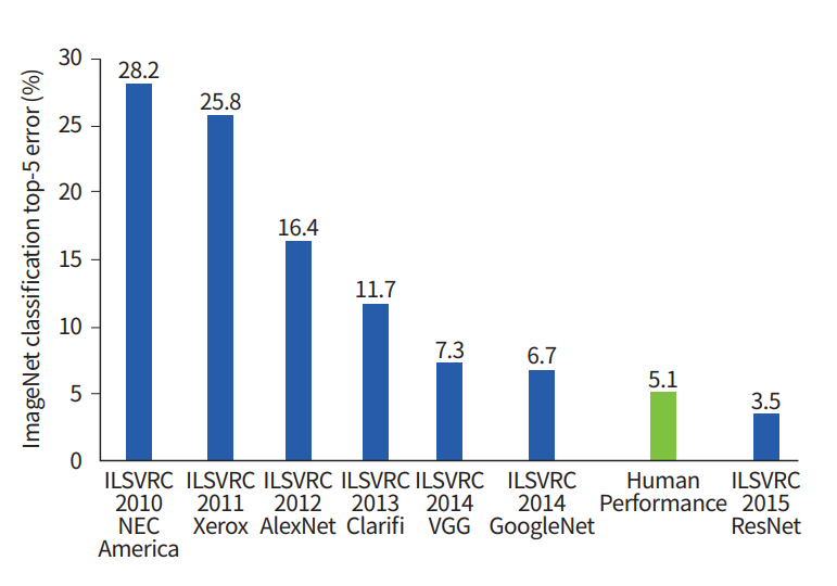
ImageNet classification performance in chronological order. ILSVRC, ImageNet Large Scale Visual Recognition Challenge.
DL has been successfully applied to many research fields and has become ubiquitous. As such, many studies have already adopted DL to improve medical imaging research, and increasingly more studies will adopt DL for medical imaging research in the future. This review article aims to survey DL literature in medical imaging and describe its potential for future medical imaging research. First, we provide an overview of how traditional machine learning evolved to DL. Second, we survey the application of DL in medical imaging research. Third, software tools for DL are reviewed. Finally, we conclude with limitations and future directions of DL in medical imaging.
FROM TRADITIONAL MACHINE LEARNING TO DEEP LEARNING
Machine learning involves building data-driven models to solve research problems [13]. There are two categories: supervised learning and un-supervised learning. In supervised learning, we train models using input data with matched labels [14]. The model is a mathematical model that can associate input data with the matched labels and a predictive model, which is validated using unseen test data. For example, we start with MRI images labeled either as a normal control or diseased, and machine learning would lead to a mathematical model that could associate MRI images with diagnosis in both training and test data. Supervised learning is commonly used in the following two tasks. In classification, the model associates input data with pre-defined categorical results (i.e., normal vs. diseased) [15-17]. The output is a discrete categorical variable in classification. In regression, the model associates input data with often continuous results (i.e., the degree of symptoms) [18]. The output is typically a continuous variable in the regression. In un-supervised learning, we use unlabeled input data to learn intrinsic patterns in the input data. Un-supervised learning is commonly used in clustering. With clustering, we might identify subgroups within a given group of patients diagnosed with the same disease. Supervised learning is more costly to prepare, as it involves annotating input data with labels, which often requires human intervention.
ANN is a statistical machine learning method inspired by brain mechanism from neuroscience (Fig. 2) [19]. Researchers designed a learning algorithm that resembles how the brain handles information. A neuron is the basic unit of the brain mechanism. The neuron is an electrically excitable cell that receives signals from other neurons, processes the received information, and transmits electrical and chemical signals to other neurons. The input signal to a given neuron needs to exceed a certain threshold for it be activated and further transmit a signal. The neurons are interconnected and form a network that collectively steers the brain mechanism. ANN is an abstraction of an interconnected network of neurons with layers of nodes, and it consists of an input layer aggregating the input signal from other connected neurons, a hidden layer responsible for training, and an output layer [20]. Each node takes the input from nodes from the previous layer using various weights and computes the activation function, which is relayed onto the next layer of nodes. The activation function approximates the complex process of a physical neuron, which regulates the strength of the neuronal output in a non-linear manner. The mathematical processing in a node can be represented using the following equation:
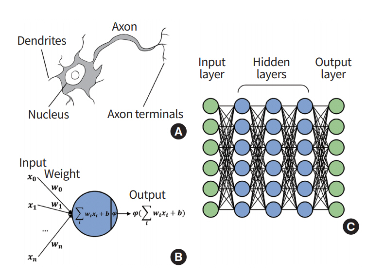
Overview of artificial neural network. (A) In a biological neuron, the nucleus transforms the chemical inputs from the dendrites into electric signals. The signals are transmitted to the next neurons through the axon terminals. (B) In a node (perceptron), the input values are transformed by the weights, biases, and activation functions. The output values are transmitted to the next perceptron. (C) Multilayer perceptron consists of multiple perceptrons.
A node takes in an input value ‘x’ and multiplies it by weight ‘W,’ and then a bias of ‘b’ is added, which is fed to the activation function ‘φ.’ Differences between the output of ANN and the target value (i.e., ground truth) are called errors or losses. The training of the ANN is a procedure to update weights that interconnect different nodes to explain the training data, which is equivalent to minimizing the loss value. The losses are back-propagated through the network, and they are used to modify the weights and biases [21,22]. As a result, components of ANN are updated to best explain the target values.
A deep neural network (DNN) is an expanded ANN incorporating many hidden layers to increase the flexibility of the model [23-26]. DNN consists of an input layer, many hidden layers, and an output layer. The added layers afford solving more complex problems but can cause other issues. The first issue is the vanishing gradient problem [27]. This occurs because the input information cannot be effectively used to update the weights of deep layers, as the information needs to travel the many layers of the activation function. This leads to under-training of the deep layers. Another issue is over-fitting, which occurs frequently when the complexity of the model increases [25]. A complex model might explain the training data well, but it does not necessarily explain the unseen test data well. The increased complexity of many layers requires a high computational load and thus degrades the training efficiency. The issues of vanishing gradient and over-fitting have been mitigated by enhanced activation function, cost function design, and drop-out approaches. The issue of the high computational load has been dealt with by using highly parallel hardware, such as GPUs and batch normalization.
Modern DL approaches employ dedicated topology of deeply stacked layers to solve a given problem. There are many variants of DL architecture, and an exhaustive review of them is outside the scope this paper. In this paper, we mention three well-known DL architectures: convolutional neural network (CNN), auto-encoder (AE), and recurrent neural network (RNN).
Convolutional neural network
CNN refers to a network architecture composed of many stacked convolutional layers [28]. Convolution is a mathematical operation based on two functions, addition and multiplication. For a given input image, convolution is applied to the input image based on a receptive filed (i.e., extents of convolution operation), which is analogous to the extents of the response region of human vision. The convolution procedure is well-suited for image recognition because it considers locally connected information (i.e., neighboring voxels or pixels). There are pooling layers between convolution layers. The pooling layer is essential to increasing the field of view of the network. It takes a portion of the locally connected nodes of the input layer and results in an output that has a smaller spatial footprint. For example, we might take the maximum value of the outputs of four neighboring nodes. It can control the over-fitting problems and reduce the computational requirements. In general, the max-pooling algorithm is used for many architectures, extracting the highest values from the receptive sliding window (Fig. 3).
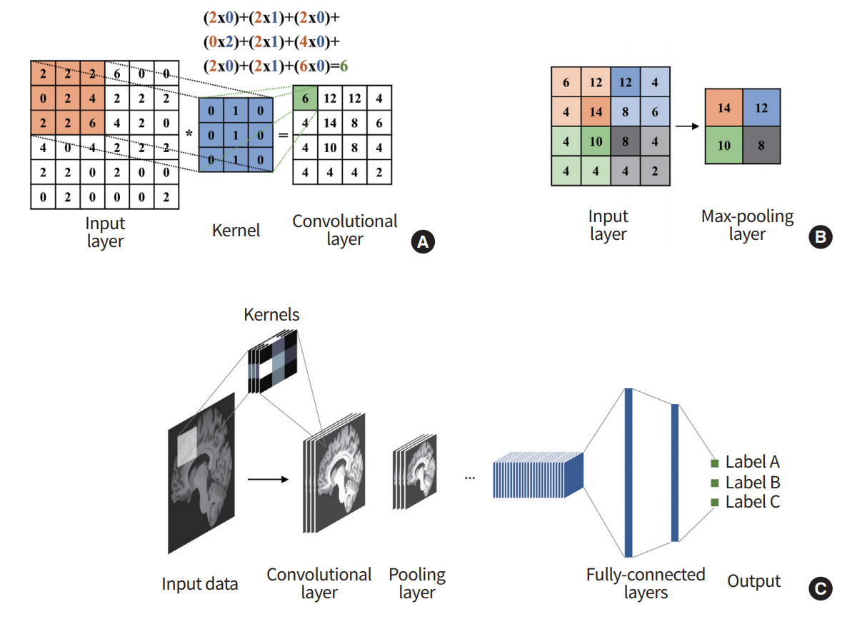
Overview of convolutional neural network (CNN). (A) The output of the convolutional layer is obtained by convolving its input layer and kernel weights. (B) The max-pooling layer outputs a down-sampled layer by extracting the maximum values from the partially windowed area of the input layer. (C) A general CNN consists of a series of convolutional layers, pooling layers, and fully connected layers.
As the last component of CNN, a series of fully connected layers follow. The fully connected layer combines all activations of the previous layers. This layer works the same as in the general ANN. After the series of fully connected layers, the model outputs the final set of feature values appropriate for the given problem. CNN was the initial catalyst for widespread adoption of DL. LeNet-5 is one of the early architectures that drastically improved existing machine learning approaches for recognizing hand-written digits [29], and there are other well-known architectures, including AlexNet, GoogLeNet, VGG-Net, and ResNET [28,30-32]. Further details of the architecture are found in the references.
Auto-encoder and stacked auto-encoder
AE is a network that is used to derive an efficient representation of the input data [33,34]. As the name suggests, this network reduces the input layers to a layer with a small number of nodes (i.e., encoding) and then restores them via the upscaling process (i.e., decoding), as shown in Fig. 4. By this process, the hidden layer can represent its input layer with a reduced dimension that minimizes the loss of input information. This model generally has an hourglass-shaped structure with a dimension of the hidden layer being smaller than the input layer.
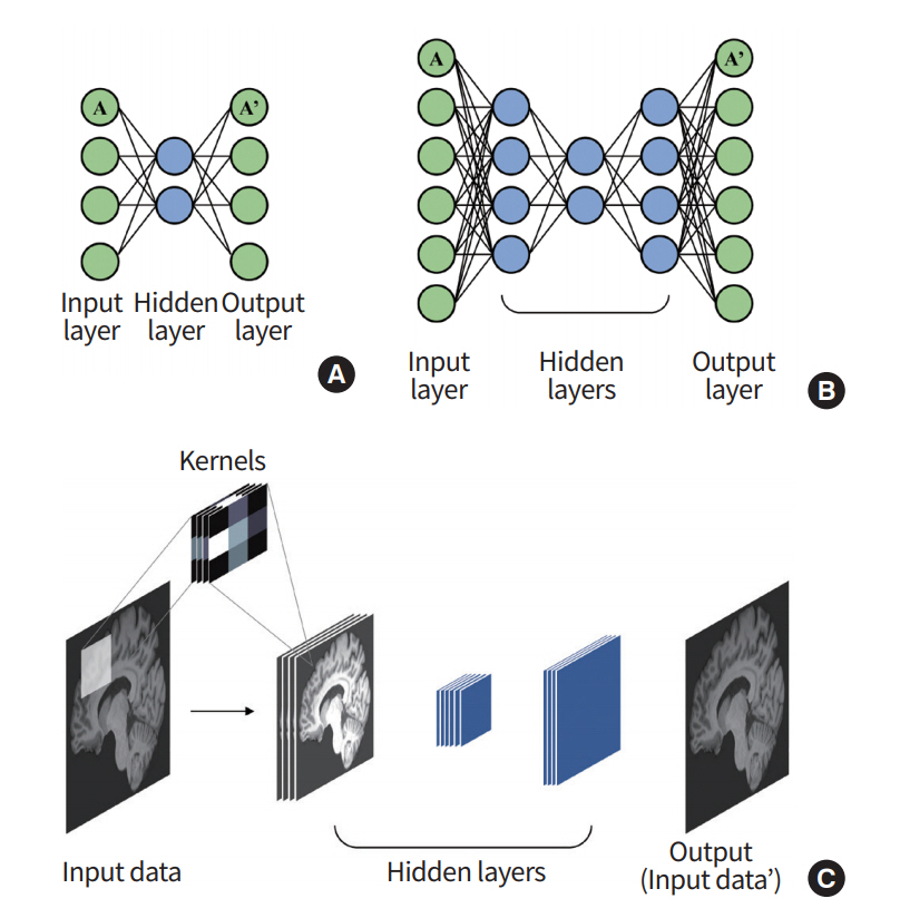
Overview of auto-encoder (AE). (A) An AE consists of multiple perceptrons that mimic the input layer. (B) A stacked auto-encoder (SAE) can be built by stacking the AEs. (C) A general SAE is trained to reconstruct the output that is similar to the given input.
Stacked auto-encoder (SAE) is made by stacking the AEs so that the output of an AE layer is treated as an input layer for another AE (Fig. 4) [35]. Vincent et al. [36] used this SAE structure to obtain a denoised image of input data. The model used the greedy training method to learn several SAEs independently.
Recurrent neural network
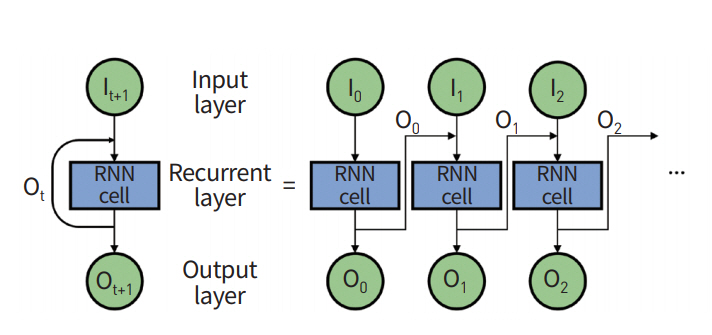
General ANN is a feed-forward network where input information starts from the input layer, travels through many hidden layers, and finally arrives at the output layer. RNN has a different topology for its layer configuration. The output of hidden layers is fed back to an input layer using feedback (Fig. 5) [37,38]. RNN considers both current input data and feedback data from previous states and thus is well-suited for modeling sequential data, including both temporal and spatial information.
DEEP LEARNING APPLICATION IN MEDICAL IMAGING
In this section, we review representative applications of DL in medical imaging. First, CADx/CADe tasks are covered with topics of classification, detection, and prediction. Second, image processing tasks are covered with topics of segmentation, registration, and generation. CADx/CADe has many critical usages in radiology, such as finding an altered structural/functional area (detection or localization), predicting the state of the object of interest based on a probabilistic model (prediction), and classifying binary or multiclass categories (classification). In contrast, image processing is the prerequisite for subsequent clinical tasks, such as diagnosis or prognosis, and they can be categorized into the following tasks: a segmentation task assigns voxels with similar properties into labels, a registration task spatially aligns two or more images onto a common spatial frame, and an enhancement task improves the image quality for the given task. Each topic is described in terms of the network architecture (e.g., CNN, RNN, or SAE) and its clinical application.
Applications using CNN architecture
CNN computes features from locally connected voxels (i.e., neighborhood voxels); hence, it is widely used as the reference model for medical image analysis. In general, a given image goes through many convolution layers, and the features are extracted from different layers. The extracted features are further used for various tasks.
CADx/CADe application using CNN architecture
CADx/CADe applications based on CNN are shown in Table 1.
Detection: The detection task refers to finding the region associated with the diseased condition. The detection task is sometimes referred to as the localization task, as it involves finding voxel positions associated with the disease. The task is often a pre-requisite for therapy planning. Many studies adopted CNN and reported precise detection performance. Dou et al. [39] applied three-dimensional (3D) CNNs to localize the lesion of cerebral microbleeds from MRI. Zreik et al. [40] proposed an automatic detection method for identifying left ventricle myocardium in coronary CT angiography using CNN. Using both PET/CT imaging, whole body multiple myeloma detection showed better performance than traditional machine learning approaches, such as the random forest classifier, k-NNs, and SVM [41]. Apart from the common imaging modalities (i.e., MRI, CT, and PET), retinal and endoscopy images, as well as histology images, were analyzed for finding the diseased region of interest (ROI) in other studies [17,42,43].
Prediction: The prediction task involves forecasting properties (often not evident to the naked eye) of an object using imaging analysis results. Prediction often occurs in a longitudinal setting, where baseline imaging findings are used to predict properties of the object in the future. Many studies attempted to compute the likelihood of clinical variables, such as drug or therapeutic response, patient’s survival, and disease grading, using imaging analysis results. Kawahara et al. [44] proposed a novel CNN framework, BrainNetCNN, to predict a cognitive and motor developmental outcome score by using structural brain networks of diffusion tensor imaging. Yasaka et al. [45] assessed the performance for predicting the staging of liver fibrosis using a CNN model on gadoxetic acid-enhanced hepatobiliary phase MRI. In the above two published papers, the predicted scores derived from CNN correlated well with the ground-truth. Some studies adopted CNN to predict treatment response [46,47]. Furthermore, CNN-based approaches have shown potential in the prediction of a patient’s survival and thus could be promising tools for precision medicine [48,49].
Classification : The classification task determines which classes the imaging data belong to. The classes could be binary (e.g., normal and diseased) or multiple categories (e.g., subclasses within the given diseased condition) depending on the task. Many studies successfully applied CNN to classify the severity of disease for different organs (i.e., brain, lung, and liver) using CT imaging [50-52]. Mohamed et al. [53] applied CNN to mammogram imaging and categorized data into a few classes proportional to breast density. Esteva et al. [54] classified skin cancer photographs into binary classes and even suggested that such operation could be performed using portable devices such as smartphones. In histology, one study showed that cell differentiation could be classified with CNN, and the results have the potential to identify tissue or organ regeneration [55].
Image processing applications using CNN architecture
Image processing applications based on CNN are shown in Table 2.
Image segmentation: The segmentation task partitions the imaging data into the target and background region. In medical imaging, this typically amounts to finding regions that are related to a disease condition (i.e., finding the tumor region). The task assigns voxels to binary classes using intensity, texture, and other derived information. Many studies successfully used CNN to segment the target region using CT and MRI for various organs, such as the brain, liver, kidney, and prostate [56-61]. Fang et al. [62] proposed an automatic segmentation algorithm of retina layer boundaries using CNN for high-resolution optical coherence tomography imaging. Xu et al. [63] adopted CNN architecture for segmenting epithelial and stromal regions in histology images.
Image registration : The image registration task spatially aligns one image with another so that both can be compared to a common spatial framework through a geometric transform. Many studies adopt multimodal imaging and thus registration is necessary to extract spatially aligned features in those studies. Registration requires a long computational time as it involves a high degree of freedom (DOF) optimization problem. The CNN-based approaches could be used as an alternative for the difficult registration problem by finding landmarks or control points through CNN architecture. Miao et al. [64] improved the registration in terms of the computation time and capture range using a real-time 2D/3D registration framework based on CNN. Another study proposed a technique for correcting respiratory motion during free-breathing MRI using CNN [65]. Yang et al. [66] introduced a novel registration framework based on CNN, Quicksilver, which performed fast predictive image registration.
Image enhancement: The image enhancement task aims to improve the image quality of the objects of interest. Depending on the application, enhancement might occur in the context of image generation or reconstruction. Nonetheless, the goal is to improve the image quality. Two studies proposed algorithms to generate a high-quality image (e.g., high dose CT) from a low quality image (e.g., low dose CT) using CNN, which reduced noise and provided more structural information than the low-quality images [67]. Image generation based on the synthesis of different modalities contributed to the improved image quality by combining the distinctive information in each modality [68,69]. Golkov et al. [70] proposed a reconstruction model based on CNN for shorter scanning time in diffusion MRI. This model allowed acceleration of the scan time and obtaining quantitative diffusion MRI. Bahrami et al. [71] explored the generation of 7 Tesla (T)-like MRI from routine 3T MRI based on CNN, where reconstructed images benefited from both resolution and contrast compared to the 3T MRI.
Applications using RNN architecture
RNN integrates results from the previous states and current input and thus is suitable for tasks involving sequential or dynamic data. In medical image analysis, spatial information is exploited using CNN, and temporal information is often exploited using RNN. Studies using dynamic imaging adopted a combination of CNN and RNN so that joint modeling of spatial and temporal information was possible references [72-77].
CAD application using RNN architecture
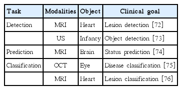
CADx/CADe applications based on RNN are shown in Table 3.
Detection: Xu et al. [72] proposed an end-to-end DL framework to accurately detect myocardial infarction at the pixel level. In this framework, the location of the heart was found based on CNN and the detected ROI was further analyzed using the dynamic cardiac MRI incorporating temporal motion information using RNN. In the same manner, Chen et al. [73] used the combined CNN and RNN for a fetal ultrasound, where ROI was found using CNN, and temporal information was processed by RNN based on the features of the ROIs in consecutive frames.
Prediction: Han and Kamdar [74] proposed convolutional recurrent neural networks (CRNN) for predicting methylation status in glioblastoma patients. In the CRNN architecture, the convolution layer extracted sequential feature vectors from each MRI slice and RNN was used to predict the methylation status integrating sequential feature information.
Classification: Gao et al. [75] designed a combined architecture of CNN and RNN for classifying the severity of nuclear cataracts in slit-lamp images, where hierarchical feature sets were extracted from CNN, and then the features were hierarchically merged into high-order image-level features. Xue et al. [76] proposed a deep multitask relationship learning network for quantifying the left ventricle in cardiac imaging, where cardiac sequence features were extracted using CNN and then temporally learned by RNN.
Image processing applications using RNN architecture
Imaging processing applications based on RNN are shown in Table 4.
Image segmentation : Zhao et al. [77] proposed a tumor segmentation method based on DL using multimodal brain MRI. They used a network composed of the combination of CNN and RNN architectures in which CNNs assigned the segmentation label to each pixel, and then RNNs optimized the segmentation result using both assigned labels and input images. Yang et al. [78] proposed an automatic prostate segmentation method using only the RNN architecture. The static ultrasound image was transformed into an interpretable sequence and then the extracted sequential data was used as input to the RNN.
Image enhancement: Qin et al. [79] suggested a framework to reconstruct high-quality cardiac MRI images from under-sampled k-space data. They adopted CRNN to improve reconstruction accuracy and speed by considering both spatial and temporal information.
Applications using SAE architecture
SAE encodes the input data using a small number of features and then decodes them back to the dimension of the original input data. In medical imaging, SAEs are commonly used to identify a compact set of features to represent the input data. The learned features could be used for specific image enhancement and reconstruction tasks.
CAD application using SAE architecture
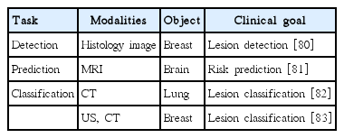
CADx/CADe applications based on SAE are shown in Table 5.
Detection: One study showed that a stacked sparse AE could be used for nuclei detection in breast cancer histopathology images [80]. This architecture could capture high-level feature representations of pixel intensity and thus enabled the classification task to be performed effectively for differentiating multiple nuclei.
Prediction: He et al. [81] adopted a variant of SAE to predict cognitive deficits in preterm infants using functional MRI data.
Classification: Chen et al. [82] proposed an unsupervised learning framework based on the convolutional AE neural network in which the patch images from raw CT were used for feature representation and classification for lung nodules. Cheng et al. [83] applied a stacked denoising AE to two different modalities, ultrasound and CT. The aim was to classify benign and malignant lesions from the two modalities.
Image processing applications using SAE architecture
Image processing applications based on SAE are shown in Table 6.
Image segmentation: Zhao et al. [84] applied SAE to learn compact feature representation from cryosection brain imaging and then classified voxels into white matter, gray matter, and cerebrospinal fluid.
Image enhancement: Janowczyk et al. [85] applied sparse AE to reduce the effects of color variation in histology images. Benou et al. [86] adopted SAE to model the spatiotemporal structure in dynamic MRI, which led to denoised MRI. The denoised MRI resulted in a more robust estimation of pharmacokinetic parameters for blood-brain barrier quantification. Some adopted SAE to generate pseudo-CT scans from MRI, which were used to reconstruct PET imaging with better tissue characteristics [87].
Among the discussed three network architectures, CNN is the most widely used. Many studies adopted CNN for various target organs (brain, lung, breast, etc.) using various imaging modalities (MRI, CT, etc.). This is partly due to the fact that CNN processes information in a hierarchical manner similar to visual processing in the human brain. RNN is typically used in conjunction with CNN, where the learned CNN features were sequentially handled through the RNN. SAE has strengths in compact feature representation, which is useful in denoising and reconstruction tasks. In summary, there is no one network structure that solves all the medical imaging problems, and thus, researchers should choose the appropriate network architecture suitable for a given problem.
SOFTWARE TOOLS FOR DEEP LEARNING
Researchers need dedicated software tools to perform DL research. Fortunately, much of the DL software is open-source; thus, the studies are more reproducible and cost effective. We review commonly used open-source DL software tools in this section.
Caffe is one of the early DL tools developed by Berkeley Vision and Learning Center [87]. The tool emphasized modularity and speed based on C++ and Python. Many early CNN works have been performed with Caffe. Researchers could easily transfer the learned models (i.e., layer structure and weights) from other research projects and use them to initialize their own DL model. Such procedures are often referred to as transfer learning, and they typically save computation time in training the model. Theano is another early DL tool [88]. Theano is Python-based and is efficient in computation using a GPU and central processing unit together.
Tensorflow is one of the most widely used tools for DL and it is backed by the internet search giant Google [89]. The Google Brain Team developed the software and it is based on Python. Users are free to leverage the vast software library available in Python. The software is well-maintained and updated frequently for additional functionality.
Torch is a DL tool that aims to facilitate the procedures to build complex models. It was originally based on non-Python Lua, but recently it added Python support via PyTorch for improved user friendliness [90].
LIMITATIONS AND FUTURE DIRECTIONS
Modern DL methods learn very high DOF models (i.e., millions of weights) from the training data. Hence, the sheer number of required training data is very high compared to conventional machine learning methods. Recent DL applications in brain MRI learned models from more than 1.2 million training data [91]. There are algorithm enhancements, such as augmentation, to artificially boost the number of training samples, but the quality of the DL methods directly rely on the number and quality of training samples. This is one of the biggest hurdles of DL research in medical imaging and is one of the reasons why large corporations such as Google can produce high-quality DL models, as they already have a huge number of training samples in-house. In medical imaging research, the large sample requirement could be partly alleviated by multisite data acquisition. Researchers need to apply a standardized protocol to acquire data so that they can be effectively combined into one set of training data for DL. Another way to boost training samples is to use an open research database. The Human Connectome Project houses thousands of high-quality brain MRI that are open to the research community. A potential issue with mixing data from different sites or research databases is the heterogeneity in image quality. One can render high-quality data into lowquality data so that all data are of similar quality. This is the practical approach because rendering low-quality data into high-quality data is difficult.
Many DL methods belong to the supervised approach; hence, they require manual labeling. Labeling thousands of imaging data by human experts is cumbersome. On top of that, inter- and intraobserver variability need to be considered, which makes the labeling procedure even more problematic. One possible way to tackle this issue is to apply a two-tiered semiautomatic approach [43]. An automatic algorithm would perform the first round of labeling and then the human experts can either accept or modify the results of the first round. Recently, one study proposed a DL method to automatically retrieve images from a large database that matched human set criterion [92-94]. This approach has the potential to be used as the initial labeling for further refinement.
Another issue related to sample size is the lack of balance in comparison groups. Many studies compare two groups: the normal control group and the diseased group. Many clinical sites have many samples of the disease group, while matched controls could be lacking. Ideally, DL algorithms require an equal number of samples in the comparison groups. If there is a large imbalance between the comparison groups, the DL algorithm would not be able to fully learn the under-represented group. A good practice is to prospectively plan research projects to avoid imbalance in comparison groups as much as possible. Many diseased conditions we explored are in fact quite heterogeneous. A given disease condition might consists of many subtypes, and more studies are aiming to dissect the differences among the subtypes. Researchers should make sure that they have appropriate labels for the subtypes and enough samples of each subtype so that DL models could be applied effectively.
DL is a highly flexible modeling approach to learn an inherent representation of the input data. It optimizes a loss function to find millions of weights that can best explain the input training data. It is very difficult to interpret how certain weights contribute to the final model. In many cases, we are left with a black box that performs the given task really well [95,96]. In traditional machine learning, we could quantify how each semantic feature contributes to the final model and better understand or improve the model as necessary. For example, we know that an irregular tumor boundary is strongly linked with malignant tumors [97,98]. However, for DL, we cannot say the n-th weight in the j-th layer has a strong link with the final outcome. Such interpretability is largely lacking in DL. Ribeiro et al. [99] proposed a novel explanation technique, local interpretable model-agnostic explanations, which performs a local approximation of the complex DL model. This algorithm carries out linear classification based on distinctive features from the simplified model, which might be interpretable. Some studies surveyed visual interpretability of various DL architectures and showed that the DL model is reliable across many domains [100-102]. There is active research tackling this interpretability issue and researchers should pay attention to future developments.
A DL algorithm requires many tuning parameters to properly train the model. The hyperparameters include learning rate, dropout rate, and kernel functions. A slight modification of these parameters might lead to drastically different models with varying performances. So far, these parameters have been chosen based on heuristic approaches relying on the experience of human experts. Active research is being performed regarding methods to automatically find optimal hyperparameters for DL. Domhan et al. [103] developed a method for automatically optimizing the hyperparameters, where the process was based on the inference of performance using a learning curve from the first few iterations. They would terminate the model, leading to bad performance based on the few initial data points. Shen et al. [104] proposed an intelligent system, including a parameter-tuning policy network, which determines the direction and magnitude for fine-tuning hyperparameters.
CONCLUSION
DL is already widespread, and it will continue to grow in the near future in all fields of science. The advent of DL is fostering new interactions among different fields. Experts in machine learning (mostly from computer science) are actively embedded in research teams to solve critical medical problems. Medical image processing will benefit immensely from DL approaches, as DL has shown remarkable performance in non-medical regular imaging research compared to conventional machine learning approaches. In this review paper, we touched on a brief history from conventional machine learning to DL, surveyed many DL applications in medical imaging, and concluded with limitations and future directions of DL in medical imaging. Despite the limitations, the advantages of DL far outweigh its shortcomings, and thus, it will be an essential tool for diagnosis and prognosis in the era of precision medicine. Future research teams in medical imaging should integrate DL experts in addition to clinical scientists in their teams so as to fully harness the potential of DL.
Notes
No potential conflict of interest relevant to this article was reported.
Acknowledgements
This work was supported by the Institute for Basic Science (grant number IBS-R015-D1) and the National Research Foundation of Korea (NRF) (grant number NRF-2016R1A2B4008545).
